Programming Assignment 1 - Device Query & Raytracer

Part 1

Objective

The purpose of this programming assignment is to familiarize the student with the underlying hardware and how it relates to the OpenCL hardware model. By extension, the program will familiarize the student with the processing resources at hand along with their capabilities. By the end of this assignment, one should understand the process of compiling and running code that will be used in subsequent modules.

All relevant code is located in the PA1 directory for this homework. For this homework, run everything on your local machine.

Instructions

The file device_query/main.c queries for devices across all platforms, and displays information about each device.

Some properties to pay attention to:

• Computational Capabilities

• Global Memory Size

• Shared Memory Size

• Work Item Size

• Work Item Dimensions

• Work Group Size

• Preferred Work Group Size Multiple

The student is encouraged to relate the device-specific information to the OpenCL memory model, provided below.

Credits: Khronos Group

How to Run

See <devcontainers> to learn how to configure devcontainers for vscode. These will create docker containers that will hold your programming environment. You should use the devcontainer for both part 1 and part 2.

The device_query/main.c file contains the host code for the programming assignment; there is no associated device kernel code for this assignment. There is a Makefile included which compiles it. It can be run by typing make from the DeviceQuery folder. It generates a device_query output file. Simply run this with ./device_query, which will print device information to the console.

Submission

You do not need to submit any code for this assignment. You must answer the questions in Gradescope.

Part 2

Objective

The second part of this assignment aims to contextualize parallelization and demonstrate the benefits of heterogenous programming. With access to multiple processing cores, multiple threads can be assigned to operate on independent tasks of a program, allowing parallelized programs to have massive benefits over their sequential counterparts.

The goal of this part of the assignment is to demonstrate the visible speedup that arises from a program running on one thread, to a program running in parallel on slightly more threads, and finally to a program that runs in parallel on many threads.

Note: You are not expected to understand what local size is for this PA.

Context

For a visually appealing example, the program chosen to desmonstrate parallelization is that of a raytracer. We first explore the high level overview of raytracer functionality to understand why parallelization is a natural application for this program.

The high level concept of raytracing is derived from the idea of shooting “rays” into a virtual world and seeing what these rays hit. One can imagine an eye shooting out into the world and being able to see whatever the ray hits. In the case of ray tracing, we have a “camera” (i.e. the eye) that produces rays starting from the eye position and going through pixels in a 2D screen.

Credits: scratchapixel.com

In the diagram above, the computer screen can be represented as a 2D grid of squares, where each square represents a pixel on the screen. A ray (labelled as primary ray) is shot from the position of the camera towards the center of the pixel.

Such a ray is created for every pixel in the screen. As such, the direction a ray goes is determined by where the origin of the ray is (that is, where the eye is positioned) and the coordinates of the pixel on the screen that the ray is shot through. In other words, every primary ray is unique to the pixel it is sent through.

On the other side of the screen is the virtual scene, composed of objects and lights. In the diagram above, we observe a singular object of a green sphere and a singular point light above it.

After the ray is created, it is sent into the virtual scene. The purpose of the ray is to probe the virtual scene. The first object in the virtual scene that the ray hits, referred to as an intersection, determines what object is closest to the screen. For simplicity, we first assume that the ray will simply track the first object intersected. As stated before, every primary ray is unique to the pixel it is sent through; as such, we may draw the color of the object that was first intersected to the screen, as an intersection of the object with the primary ray indicates that we can see the object.

In the diagram below, we can see that an intersection of a primary ray (referred to as a view ray in the below diagram) with the blue sphere in the scene results in blue being drawn to the pixel that the primary ray goes through. In other words, the job of a ray in a ray tracer is to simply probe the scene to determine which color to draw at each pixel.

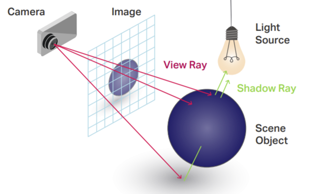
Credits: Graphic Speak

In a raytracer, a primary ray is drawn through every pixel. As such, the psuedocode would look something like this:

for x in image_width:
  for y in image_height:
    create ray through pixel (x, y)
    get color and display color on pixel (x, y)

And that’s the (very) high level overview of how a raytracer works! Of course, there’s a lot of processing and nested for-loops within the process of getting a color (iterating through objects in a scene), all the lights, etc.). So how does parallelization fit into this?

Recall that a primary ray is a property of the pixel in the screen that it is sent through. That is to say, every ray that is sent through a piel determines that pixel color independently!

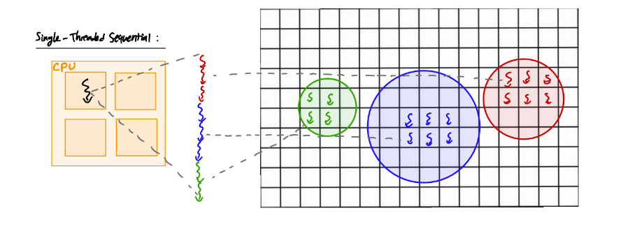
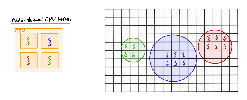
The current implementation based on the psuedocode runs only on a single thread on one processor, and relies on nested for-loops to iterate through every pixel in the screen. What if we had multiple processors we could use at once, thus producing multiple rays simultaneously?

Thus, we can parallelize the generation of rays in a raytracer, an application of parallel computing so simple that it is considered embarassingly parallel :)

With the context out of the way, let’s dive into the code!

Instructions

The code for a basic sequential raytracer has already been provided as well as the kernel for the parallel raytracer. The goal of this part is not to have you be able to write your own raytracer from scratch, but to understand its overall structure of OpenCL host code and see how it can be parallelized. By extension, to demonstrate how effective parallelization can be!

Step 1:

The first program to look at is in the raytracer_sequential directory. Here, open up raytracer_sequential/main.c. This is the implementation of a raytracer for a single-threaded program running on the CPU. Given that there is only one thread, the naive implementation of iterating through every pixel is used, resulting in a nested for loop. Scan through this code and understand where this for-loop is located and how it is used to determine which pixel is being drawn to.

On the DSMLP OpenCL can only access the CPU if the environment variable POCL_DEVICES is unset. If you have already set it, you can unset it with unset POCL_DEVICES.

Step 2:

Now, run the program using the command make run. This will compile the program and generate an output file output.png. You can view this file to see a neat little scene that the program generated! You’ll also notice in the terminal that the time it took for the program to run was also outputted. Note how much time the sequential implemenation of the raytracer took! We’ll see how our next implemenation compares.

Step 3:

Now that we have a benchmark performance of how long a sequential, single-threaded implemenation of a raytracer on the CPU is, let’s compare it with a parallelized implemenation! You can find the kernel (the program meant to run on a compute device) in the directory raytracer_parallel as a file titled kernel.cl. This is an OpenCL kernel. Compare this with raytracer_sequential/main.c in the sequential implementation; what do you notice (hint: what happened to the for-loop? Why might this be?).

Step 4:

The kernel doesn’t actually run by itself; instead, it needs to be built by some main program that will read the kernel program as a string and build the correct context and command queues to map the kernel to a compute device and run it. This is done in raytracer_parallel/main.c.

Implement the arguments needed in order to build the correct context and command queue and free memory. Everything that needs your attention in the raytracer_parallel/main.c marked with //@@. See the OpenCL documentation for how to fill out these arguments.

What’s nice about kernels in OpenCL is that they can be mapped to any compute device (in theory), whether that be a CPU, a GPU, even an FPGA. That’s great for us! Depending on Operating system support, we can try running the kernel on a variety of devices.

Recall from Part 1 that each device that OpenCL recognizes on your computer is associated with an index. Typically a computer will have a device for the GPU and may have a device for the GPU. Try running the parallel raytracer on the devices available on your system with raytracer_parallel gpu/cpu (make cpu or make gpu also work).

On the DSMLP OpenCL can only access the GPU (and not the CPU) if the environment variable POCL_DEVICES is set to cuda. This can be set with export POCL_DEVICES=cuda.

Recap

We have two programs:

• Sequential implementation (raytracer_sequential/main.c)

• Kernel implementation (raytracer_parallel/main.c and raytracer_parallel/kernel.cl), raytracer_parallel/main.c needs to be implemented.

The sequential implementation runs on a single thread on the CPU.

The Kernel implemenation will run on the GPU. Depending on your computer, it may also run on the CPU. Depending on the device, the number of cores accessible (and thus the number of active threads) differs. This causes differences in performance; that is, the more threads we have access to, the greater the degree of parallelization.

From this example, you should have been able to witness firsthand the power of parallelization!

Submission

Submit the raytracer_parallel/main.c. You must answer the questions in Gradescope.